Periodic Systems: Spring-2026
HW 6 (SOLUTION): Due Day 15
- Momentum of a Free Particle
S1 5497S
Consider a free particle whose wave function is \(\psi(x) = A\sin(p_0x/\hbar)\),
Is this wave function an eigenstate of momentum?
First I notice that the sine function can we written as a linear combination of complex exponentials: \begin{eqnarray*} \psi(x) &=& A\frac{1}{2i}(e^{ip_0x/\hbar}-e^{-ip_0x/\hbar}) \end{eqnarray*}
Each term is an eigenfunction, with eigenvalues \(p_0\) and \(-p_0\). Since the eigenvalues are different, this linear combination is not an eigenfunction. I can check that by letting the momentum operator act on the function to see if I get the same function back again with a multiplicative constant:
\begin{align*} \hat{p}\psi(x) &= -i\hbar\frac{\partial}{\partial x} A \sin(p_0x/\hbar) \\ &= -i\hbar\Bigg(A\cos\Big(\frac{p_0x}{\hbar}\Big)\frac{p_0}{\hbar}\Bigg) \\ &= -ip_0(A\cos\Big(\frac{p_0x}{\hbar}\Big) \end{align*}
So, no - not an eigenfunction of momentum.
What are the possible results of a measurement of the momentum?
I can rewrite this state in Dirac notation
\[|\psi\rangle = C(|p_0\rangle-|-p_0\rangle)\]
Namely, I would measure momentum to be \(p_0\) or \(-p_0\) at equal probability of 50%.
Calculate the expectation value \(\langle p\rangle\) and uncertainty \(\Delta p\) of momentum.
So the expectation value (i.e., average) is
\[\langle \hat{p} \rangle = 0.5p_0 + 0.5(-p_0) = 0\]
and the uncertainty (i.e., standard deviation) is
\[\Delta p = \sqrt{\langle p^2 \rangle - \langle p\rangle^2} = \sqrt{p_0^2-0} = p_0\]
- Dispersion Relation of a Free Particle
S1 5497S
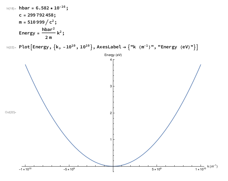
For a 1-D free particle, whose wave function is \(\psi(x) = Ae^{ikx}\), plot its dispersion relation, namely: the energy as a function of wave vector \(k\). Note \(k\) can be positive or negative. (The dispersion relation will come back later in the course.)
Using the energy eigenvalue equation on this state, we get: \begin{align} \hat{H}\psi&=-\frac{\hbar^2}{2m} \frac{\partial^2\psi}{\partial x^2}\\ &=\frac{\hbar^2}{2m}k^2(Ae^{ikx})\\ &=\frac{\hbar^2}{2m}k^2\psi=E\psi \end{align} So this will look like a parabolic function \(E= \frac{\hbar^2}{2m} k^2\).
One way to plot is in Mathematica, as shown below.
- Position and Momentum Commutation
S1 5497S
Calculate the commutator of the position and momentum operators. Do this two ways:
using the position representation of the operators
To find the commutator of \(\hat x\) and \(\hat p\), we need to find the result of operating both operators in either order.
\begin{align*} \hat x \hat p \phi(x) &= -i \hbar x \frac{d\phi}{dx} \\ \hat p \hat x \phi(x) &= -i \hbar \frac{d}{dx}\left(x\phi(x)\right) \\ &= -i\hbar \phi(x) - i\hbar x \frac{d\phi}{dx} \\ [\hat x,\hat p]\phi &= \hat x \hat p \phi - \hat p \hat x \phi \\ &= -i \hbar x \frac{d\phi}{dx} - \left(-i\hbar \phi(x) - i\hbar x \frac{d\phi}{dx}\right) \\ &= i\hbar\phi \\ [\hat x,\hat p] &= i\hbar \end{align*}
using the momentum representation of the operators
We can also do this in momentum space \begin{align*} \hat p \hat x \tilde\phi(p) &= i \hbar p \frac{d\tilde\phi}{dp} \\ \hat x \hat p \tilde\phi(p) &= i \hbar \frac{d}{dp}\left(p\tilde\phi(p)\right) \\ &= i\hbar \tilde\phi(p) + i\hbar p \frac{d\tilde\phi}{dp} \\ [\hat p,\hat x]\tilde\phi &= \hat p \hat x \tilde\phi - \hat x \hat p \tilde\phi \\ &= i \hbar p \frac{d\tilde\phi}{dp} - \left(i\hbar \tilde\phi(p) + i\hbar p \frac{d\tilde\phi}{dp}\right) \\ &= -i\hbar\tilde\phi \\ [\hat x,\hat p] &= i\hbar \end{align*}
Either way we get the same result, \(i\hbar\).
Incidentally, you might be wondering why an algebraic combination of Hermitian operators gives us something imaginary. (Or you might not...)
If you take a Hermitian conjugate of a commutator:
\begin{align*} [A,B]^{\dagger} &= (AB - BA)^\dagger \\ &= (AB)^\dagger - (BA)^\dagger \\ &= B^\dagger A^\dagger - A^\dagger B^\dagger \\ &= BA - AB \\ &= -[A,B] \end{align*}
Notice, this result is that the commutator is not a Hermitian operator. This could seem weird, since “normally” arithmetic combinations of Hermitian operators give Hermitian operators. The exception to that rule is precisely when operators that are multiplied fail to commute.
- Derivatives of the Gaussian
S1 5497S
The normalized Gaussian function is of the form
\[f(x)=\frac{1}{\sqrt{2\pi}\sigma} \,e^{-\frac{(x-x_0)^2}{2\sigma^2}}\]
- Find the first two derivatives of the Gaussian function, by hand.
\begin{align*} f(x)&=\frac{1}{\sqrt{2\pi}\sigma} \, e^{-\frac{(x-x_0)^2}{2\sigma^2}}\\ f'(x)&=\frac{1}{\sqrt{2\pi}\sigma} \, e^{-\frac{(x-x_0)^2}{2\sigma^2}} \left[-\frac{x-x_0}{\sigma^2}\right]\\ f''(x)&=\frac{1}{\sqrt{2\pi}\sigma} \, e^{-\frac{(x-x_0)^2}{2\sigma^2}} \left[\left(-\frac{x-x_0}{\sigma^2}\right)^2 -\frac{1}{\sigma^2}\right]\\ &=\frac{1}{\sqrt{2\pi}\sigma} \, e^{-\frac{(x-x_0)^2}{2\sigma^2}} \left[\frac{1}{\sigma^4}\left((x-x_0)^2-\sigma^2\right)\right]\\ \end{align*} Don't forget to use the product rule in the second derivative.
- Make a table describing where the signs of the Gaussian itself and the signs of its first two derivatives are positive and negative.
Notice that a exponential function with a real-valued exponent is always strictly positive. Therefore, the Gaussian function itself is always strictly positive and the first and second derivatives of the Gaussian function are positive or negative or zero depending on the sign of the factor multiplying the “Gausssian” part of the expressian. Of course, these are all continuous functions, so any time one of them changes sign, its value goes to zero.
\(x<x_0-\sigma\) \(x_0-\sigma<x<0\) \(0<x<x_0+\sigma\) \(x>x_0+\sigma\) \(f(x)>0\) \(f(x)>0\) \(f(x)>0\) \(f(x)>0\) \(f'(x)>0\) \(f'(x)>0\) \(f'(x)<0\) \(f'(x)<0\) \(f''(x)>0\) \(f''(x)<0\) \(f''(x)<0\) \(f''(x)>0\) - Use your table to describe the shape of the Gaussian function.
The first derivative tells us the slope of the tangent line to the original Gaussian function. We see that it is positive for \(x<x_0\) and negative for \(x>x_0\). This derivative tells us that the original Gaussian function increases until \(x=x_0\), and decreases thereafter.
The sign of the second derivative tells us if the original Gaussian function is concave up (positive second derivative) or concave down (negative second derivative). We see that the orignal Gaussian is concave down for the “distance” \(\sigma\) around \(x_0\) and concave up outside this region. The points \(x=x_0\pm\sigma\) are inflection points where the second derivative is zero and the function switches concavity.
- Find the first two derivatives of the Gaussian function, by hand.