Periodic Systems: Spring-2026
HW 7 (SOLUTION): Due Day 18
- Width of momentum-space and position-space wavepackets
S1 5498S
Consider a momentum-space Gaussian:
\[ \phi(p) = \Bigg(\frac{1}{2\pi\beta^2}\Bigg)^{1/4} e^{-(p-p_0)^2/4\beta^2}\]
Calculate the corresponding position-space wavefunction.
To find the position space wavefunction, I take the Fourier transform:
\begin{align*} \psi(x) &= \left\langle {x}\middle|{\psi}\right\rangle \\ &= \left\langle {x}\right|\Big(\int_p \left|{p}\right\rangle \left\langle {p}\right|dp \Big)\left|{\psi}\right\rangle \\ &=\int_p \left\langle {x}\middle|{p}\right\rangle \left\langle {p}\middle|{\psi}\right\rangle dp \\ &=\int_p \frac{e^{ipx/\hbar}}{\sqrt{2\pi\hbar}}\phi(p)\;dp \\ &=\frac{1}{\sqrt{2\pi\hbar}}\Bigg(\frac{1}{2\pi\beta^2}\Bigg)^{1/4}\int_{-\infty}^{\infty} e^{ipx/\hbar}e^{-(p-p_0)^2/4\beta^2}\;dp \\ &=\frac{1}{\sqrt{2\pi\hbar}}\Bigg(\frac{1}{2\pi\beta^2}\Bigg)^{1/4}\Bigg( 2\beta\sqrt{\pi}e^{-\beta^2x^2/\hbar^2}e^{ixp_0/\hbar}\Bigg) \\ \end{align*}
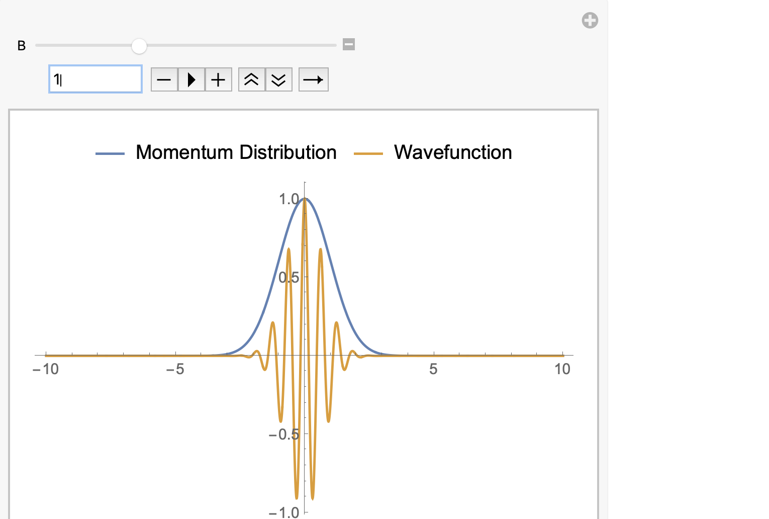
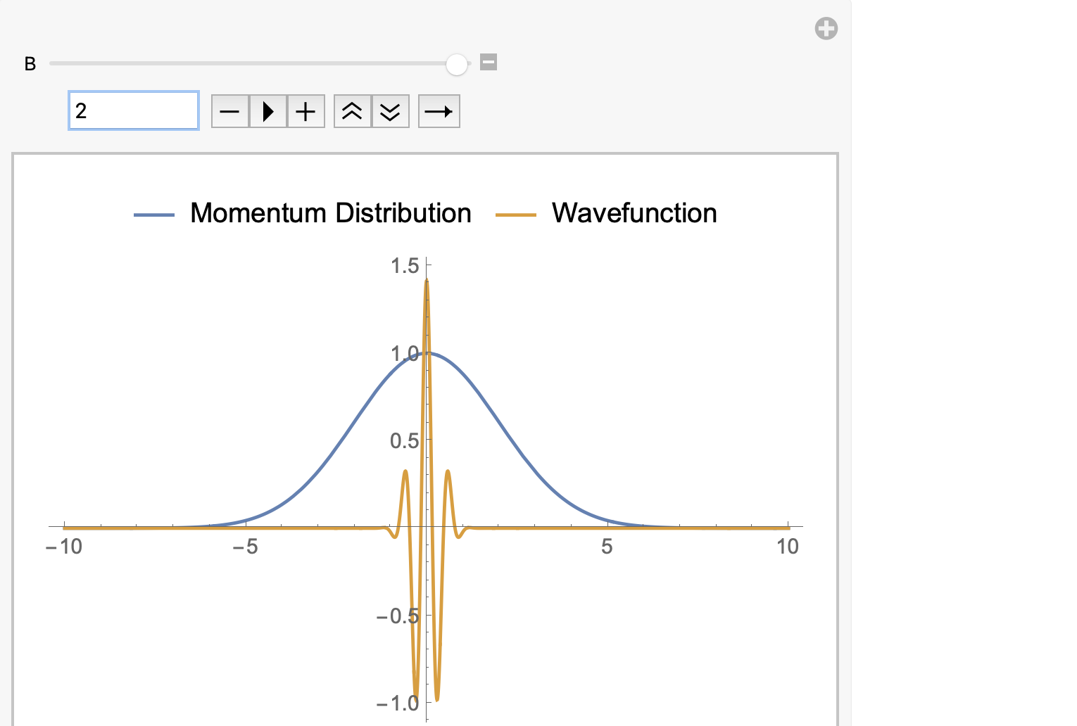
Use your favorite computational plotting tool to plot the momentum-space distribution and the position-space wavefunction. How are the widths of these two distributions related to each other? Include some plots to demonstrate the variation.
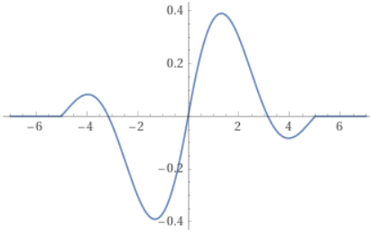
If I plot the real part of the wavefunction, I see a position wavepacket. For the purposes of comparison, I'll plot the momentum distribution and the wavefunction on the same axes:
The important bits are the exponentials. Comparing the equation for the envelope with the original momomentum distribution and generic equation for a Gaussian function: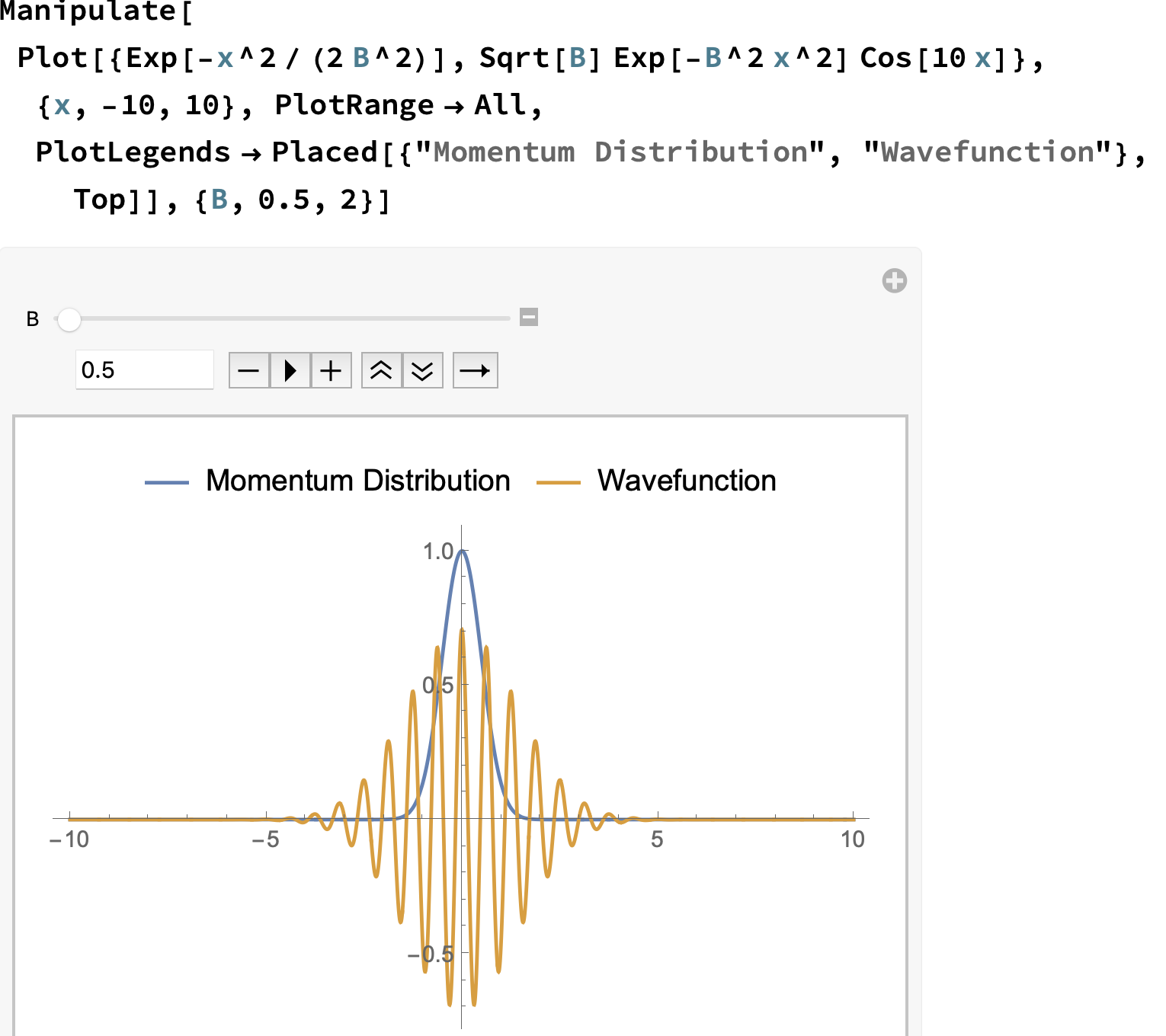
\begin{align*} e^{-\color{red}{\beta^2}x^2/\color{red}{\hbar^2}} \leftrightarrow e^{-(x-x_0)^2/2\color{red}{\sigma^2}}\\ e^{-(p-p_0)^2/2\color{blue}{\beta^2}} \leftrightarrow e^{-(x-x_0)^2/2\color{blue}{\sigma^2}} \end{align*}
I see that the width of momentum distribution is \(\beta\) and the width of wavepacket envelope is \(\hbar^2/2\beta^2\). As the momentum distribution gets narrower (\(\beta\) decreases), then the wavepacket gets wider.
- Momentum-Space Probability Distribution
S1 5498S
A beam of particles is described by the wave function:
\[\psi(x) = \begin{cases} Ae^{ip_0x/\hbar}(b-|x|) & |x|<b \\ 0 & |x| > b\end{cases}\]
where \(b>0\).
Normalize the wave function.
To normalize, integrate the norm square and set equal to 1:
\begin{align*} 1 &= \int_{-\infty}^{\infty}|\psi(x)|^2dx \\ &= \int_{-b}^{b}|Ae^{ip_0x/\hbar}(b-|x|)|^2\;dx \\ &= 2\int_{0}^{b}|Ae^{ip_0x/\hbar}(b-x)|^2\;dx \\ &= 2\int_{0}^{b}|A|^2 (b^2-2bx+x^2)\;dx \\ &= 2|A|^2 \Big(b^2x-bx^2+x^3/3\Big)\Big|_0^b \\ &= 2|A|^2 \Big(b^3-b^3+b^3/3-0+0 -0\Big) \\ &= 2|A|^2b^3/3 \\ |A| &= \sqrt{\frac{3}{2b^3}} \end{align*}
\[\psi(x) = \begin{cases} \sqrt{\frac{3}{2b^3}}\;e^{ip_0x/\hbar}(b-|x|) & |x|<b \\ 0 & |x| > b\end{cases}\]
Plot the real and imaginary parts of the wavefunction.
Separating this out into real and imaginary parts: \[\psi(x) = \begin{cases} \sqrt{\frac{3}{2b^3}}\;\left(\cos\left(\frac{p_0x}{\hbar}\right)+i\sin\left(\frac{p_0x}{\hbar}\right)\right)(b-|x|) & |x|<b \\ 0 & |x| > b\end{cases}\] Now we can easily plot this (\(b=5\)):
Real part of \(\psi\)
Imaginary part of \(\psi\)
Plot the position probability density.
The probability density is the norm square of the wavefunction:
\begin{align*} |\psi(x)|^2 &= \begin{cases} \frac{3}{2b^3}|(b-|x|)|^2 & |x|<b \\ 0 & |x| > b\end{cases} \\ &= \begin{cases} \frac{3}{2b^3}(b^2+2bx+x^2) & -b<x<0 \\ \frac{3}{2b^3}(b^2-2bx+x^2) & 0<x<b \\ 0 & |x| > b\end{cases} \end{align*} Now we can plot this (\(b=5\)):
Calculate and plot the momentum probability distribution.
The momentum space wavefunction is calculated by taking the Fourier Transform of the position space wavefunction:
\begin{align*} \phi(p) &= \int_{\infty}^{\infty} \left\langle {p}\middle|{x}\right\rangle \left\langle {x}\middle|{\psi}\right\rangle dx \\ &= \int_{-\infty}^{\infty} \frac{e^{-ipx}}{\sqrt{2\pi\hbar}} \left\langle {x}\middle|{\psi}\right\rangle dx \\[10pt] &= \int_{-b}^0 \frac{e^{-ipx/\hbar}}{\sqrt{2\pi\hbar}}\sqrt{\frac{3}{2b^3}}\; e^{ip_0x/\hbar}(b+x)\;dx + \int_{0}^b \frac{e^{-ipx\hbar}}{\sqrt{2\pi\hbar}}\sqrt{\frac{3}{2b^3}}\; e^{ip_0x/\hbar}(b-x)\;dx \\[10pt] &= \frac{1}{\sqrt{2\pi\hbar}}\sqrt{\frac{3}{2b^3}}\Big(\int_{-b}^0 e^{-ipx/\hbar}e^{ip_0x/\hbar}(b+x)\;dx + \int_{0}^b e^{-ipx/\hbar}\; e^{ip_0x/\hbar}(b-x)\;dx\Big) \\[10pt] &= \frac{3}{\sqrt{4\pi\hbar b^3}}\Big(\int_{-b}^0 e^{-i(p-p_0)x/\hbar}(b+x)\;dx + \int_{0}^b e^{-i(p-p_0)x/\hbar}(b-x)\;dx\Big) \\[10pt] &= \frac{3}{\sqrt{4\pi\hbar b^3}}\frac{2\hbar^2(\cos\frac{p-p_0}{\hbar}-1)}{(p-p_0)^2} \\[10pt] \end{align*}
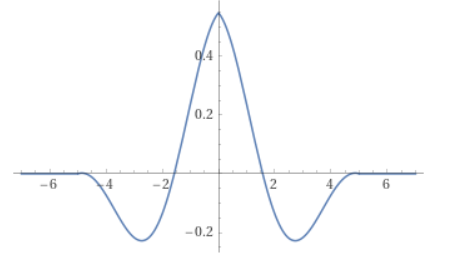
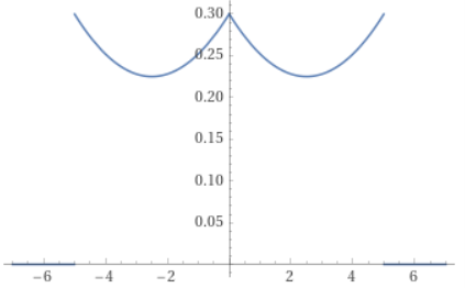
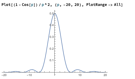
Forgetting the scaling factors, the shape of the momentum wavefunction is:
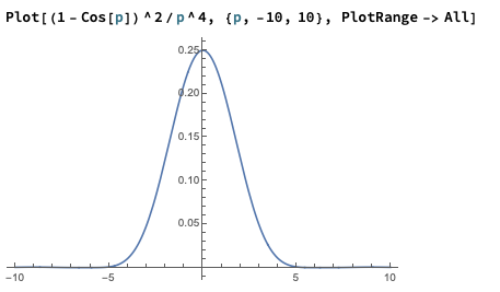
The probability density in momentum space is the norm square:
- Estimate Ground State Energy of the Hydrogen Atom
S1 5498S
Use the uncertainty principle to estimate the ground state energy of the hydrogen atom.
I'll start by writing the energy of the hydrogen atom system using a Coulomb potential:
\[E = \frac{p^2}{2m} - \frac{ke^2}{r}\]
where \(e\) is the magnitude of the charge of an electron/proton.
Next, I'll minimize the uncertainty relation between the momentum and the position:
\[ \Delta p = \frac{\hbar}{2\Delta r}\]
Plugging into the energy and changing the radial position to be the uncertainty in the radial position:
\[E = \frac{\hbar^2}{8m\Delta r^2} - \frac{ke^2}{\Delta r}\]
In plugging this in, we made the decision to equal \(r\) and \(p\) with their uncertainties, which may seem odd, but since this is an approximation we only really care if the values in question are near each other in magnitude and it turns out this is often the case for the ground state, at least enough to get us a ballpark estimate.
Now I'll minimize the energy with respect to \(\Delta r\):
\begin{align*} 0 &=\frac{dE}{d\Delta r} \\ &= -\frac{\hbar^2}{4m\Delta r^3} + \frac{ke^2}{\Delta r^2} \\ \Delta r &= \frac{\hbar^2}{4mke^2} \end{align*}
Plugging this length into the energy:
\begin{align*} E &= \frac{\hbar^2}{8m(\frac{\hbar^2}{4mke^2})^2} - \frac{ke^2}{\frac{\hbar^2}{4mke^2}} \\ &= \frac{2mk^2e^4}{\hbar^2} - \frac{4mk^2e^4}{\hbar^2} \\ &= -\frac{2mk^2e^4}{\hbar^2} \end{align*}
Plugging in numbers:
\begin{align*} m_e &= 9.1 \times 10^{-31} \mbox{ kg} \\ e &= 1.6 \times 10^{-19} \mbox{ C} \\ k &= 9 \times 10^9 \mbox{ Nm}^2\mbox{/C}^2 \\ \hbar &= 1.05 \times 10^{-34} \mbox{ m}^2 \mbox{kg/s} \\ E &= -\frac{2(9.1 \times 10^{-31} \mbox{ kg})(9 \times 10^9 \mbox{ Nm}^2\mbox{/C}^2)^2(1.6 \times 10^{-19}\mbox{ C})^4}{(1.05 \times 10^{-34} \mbox{ m}^2 \mbox{kg/s}} \\ &= -8.8 \times 10^{-18} \mbox{ J} \\ &= -55 \mbox{ eV} \end{align*}
The exact answer is \(-13.6\) eV, so this estimate gets me to within a factor of 4.