Periodic Systems: Spring-2026
HW 8 (SOLUTION): Due Day 20
- Ground‑State Uncertainty in an Infinite Potential Well
S1 5499S
Consider a particle confined in a one‑dimensional infinite square potential well of width \(L\), defined by the potential \begin{align*} V = \begin{cases} \infty & x< 0\\ 0 & 0 \leq x \leq L \\ \infty & L<x \end{cases} \end{align*}
The normalized ground-state wavefunction of the particle is \begin{equation*} \psi(x)=\sqrt{\frac{2}{L}}\sin\left(\frac{\pi x}{L}\right), \hspace{1cm} 0\le x \le L. \end{equation*}
Calcluate the postion uncertainty \(\Delta x\) and the momentum uncertainty \(\Delta p\) for the ground state of the particle, and confirm that \(\Delta x \Delta p > \frac{\hbar}{2}.\)
:
Position uncertainty \(\Delta x\)
Expectation values \begin{equation*} \langle\hat{x}\rangle = \int^L_0x|\psi(x)|^2 dx = \frac{2}{L}\int^L_0x\sin^2\left(\frac{\pi x}{L}\right) dx =\frac{L}{2} \end{equation*} \begin{equation*} \langle\hat{x}^2\rangle = \frac{2}{L}\int^L_0x^2 \sin^2\left(\frac{\pi x}{L}\right) dx =L^2\left(\frac{1}{3}-\frac{1}{2\pi^2}\right) \end{equation*}
Uncertainty \begin{equation*} \Delta x=\sqrt{\langle\hat{x}^2\rangle-\langle\hat{x}\rangle^2} =L\sqrt{\frac{1}{12}-\frac{1}{2\pi^2}} \end{equation*}
Numerically, \(\Delta x \approx0.180L\)
Momenum uncertainty \(\Delta p\)
We can compute the expectation values using the momentum operator: \begin{equation*} \hat{p}=-i\hbar\frac{d}{dx} \end{equation*}
Because the wavefunction is real and symmetric about the center, \begin{equation*} \langle\hat{p}\rangle = 0 \end{equation*}
The energy expectation value is the ground state energy: \begin{equation*} \langle\hat{H}\rangle=\left\langle\frac{\hat{p}^2}{2m}\right\rangle = E_1 \Rightarrow \langle\hat{p}^2\rangle = 2mE_1, \end{equation*} where \begin{equation*} E_1 =\frac{\pi^2\hbar^2}{2mL^2} \end{equation*} Thus, \begin{equation*} \langle\hat{p}^2\rangle = \frac{\pi^2\hbar^2}{L^2} \end{equation*}
Uncertainty \begin{equation*} \Delta p=\sqrt{\langle\hat{p}^2\rangle-\langle\hat{p}\rangle^2} =\frac{\pi\hbar}{L} \end{equation*}
Uncertainty product \begin{equation*} \Delta x \Delta p =\hbar\pi \sqrt{\frac{1}{12}-\frac{1}{2\pi^2}} \approx0.568\hbar>\frac{\hbar}{2} \end{equation*}
- Reflection from a Square Barrier
S1 5499S
Consider a particle with mass \(m\) and energy \(E\) incident from the left on a square potential barrier with height \(V_0>0\): \begin{equation*} V(x) = \begin{cases} 0 & x<0 \\ V_0 & 0<x<a\\ 0 & a<x \end{cases} \end{equation*}
This is an example of an unbounded system, so there is no condition on the energy eigenvalue. There are two cases, \(E>V_0\) and \(E<V_0\). Consider only \(E>V_0\).
Set up a wave incident from the left, and one transmitted to the right, so the total wave function is:
\begin{equation*} \psi(x) = \begin{cases} e^{ik_1x} + Ae^{-ik_1x} & x<0 \\ Ce^{ik_3x} + De^{-ik_3x} & 0<x<a \\ Be^{ik_2x} & a<x\\ \end{cases} \end{equation*}
Use the energy eigenvalue equation to solve for the values \(k_1\), \(k_2\), \(k_3\) in terms of \(E\) and \(V_0\).
Our picture and where these wave terms come from look like this:
We expext standing wave solutions inside the bump and travelling waves everywhere else. With the incident wave from the left having coefficent 1 since it is composed of 100% of our particles. Now we use the Energy Eigenvalue equation for each region, starting with region 1 (before the bump): \begin{align} \hat{H}\psi+V\psi=E\psi\\ -\frac{\hbar^2}{2m}\frac{\partial^2\psi}{\partial x^2}+V\psi=E\psi \end{align} In region 1, we have the wavefunction \(e^{ik_1x} + Ae^{-ik_1x}\) and \(V=0\), so we plug these in and take 2 derivatives: \begin{align} -\frac{\hbar^2}{2m}\frac{\partial^2\psi}{\partial x^2}+V\psi=E\psi\\ -\frac{\hbar^2}{2m}\frac{\partial^2}{\partial x^2}\left(e^{ik_1x} + Ae^{-ik_1x}\right)=E\psi\\ -\frac{\hbar^2}{2m}(ik_1)\frac{\partial}{\partial x}\left(e^{ik_1x} - Ae^{-ik_1x}\right)=E\psi\\ -\frac{\hbar^2}{2m}(ik_1)^2\left(e^{ik_1x} + Ae^{-ik_1x}\right)=E\psi\\ \frac{\hbar^2k_1^2}{2m}\psi=E\psi\\ E=\frac{\hbar^2k_1^2}{2m}\rightarrow k_1=\sqrt{\frac{2mE}{\hbar^2}} \end{align} W can do this again for the region after the bump, but despite having only one exponential, we would get the exact same answer with a different \(k\), namely: \begin{align} k_2=\sqrt{\frac{2mE}{\hbar^2}} \end{align} The only difference inside the bump is that we have \(V=V_0\) and so that term survives, but it is just a constant next to \(\psi\), just like the term \(E\psi\) and so we can group them together and follow along the math and get a similar answer except \(E-V_0\) replaces the \(E\) in our other \(k\)'s: \begin{align} k_3=\sqrt{\frac{2m(E-V_0)}{\hbar^2}} \end{align} For simplicity, we will just call the two \(k\)'s that are the same \(k\) and the duifferent one \(q\), so: \begin{align} k_1=k_2=k=\sqrt{\frac{2mE}{\hbar^2}} \\ k_3 = q = \sqrt{\frac{2m(E-V_0)}{\hbar^2}} \end{align}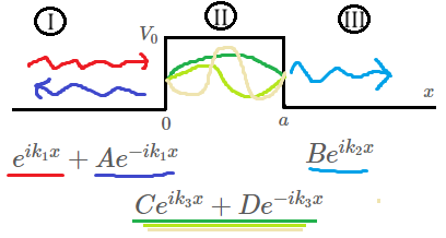
What are the boundary conditions that establish the relationship among the coefficients \(A\), \(B\), \(C\), and \(D\)?
The continuity of wave function and its first derivative is all I need. For continuity at \(x=0\) we plug 0 in for \(x\) in \(e^{ikx} + Ae^{-ikx}\) and \(Ce^{iqx} + De^{-iqx}\) and set them equal (ensuring they will be equal on the boundary), doing so we get: \begin{align} 1+A = C+D \end{align} Doing the same thing, but for the derivatives of those two functions, we get: \begin{align} ik(1-A) = iq(C-D) \end{align} Then we do the same conditions at the other boundary at \(x=a\), which gives us continuity of the wave function and its derivative at that boundary, and we get: \begin{align} Ce^{iqa}+De^{-iqa} = Be^{ika}\\ iq(Ce^{iqa}-De^{-iqa}) = ikBe^{ika} \end{align} So in total, our boundary coniditions give us a system of equations to solve which looks like this: \begin{eqnarray} 1+A &=& C+D\\ Ce^{iqa}+De^{-iqa} &=& Be^{ika}\\ ik(1-A) &=& iq(C-D)\\ iq(Ce^{iqa}-De^{-iqa}) &=& ikBe^{ika} \end{eqnarray}
The probability to observe the particle reflected is \begin{equation*} r \equiv \left|A\right|^2 \end{equation*} (remember we measure probabilities, and not amplitudes). Find \(r\). Also find the probability of transmission
\begin{equation*} t \equiv \left|B\right|^2 \end{equation*}
To make the algebra easy, you can assume that \(E=\frac{4}{3}V_0, \,V_0=\frac{3}{8m}(\frac{2\pi\hbar}{a})^2\).
Show that \(r+t=1\).
Given the special values of energy and potential, we can easily find \(k=\frac{2\pi}{a}\), and \(q = \frac{\pi}{a}\). Therefore we have
\begin{align*} 1+A &= C+D\\ C(-1)+D(-1) &= B\\ i\frac{2\pi}{a}(1-A) &= i\frac{\pi}{a}(C-D)\\ i\frac{\pi}{a}[C(-1)-D(-1)] &= i\frac{2\pi}{a}B \end{align*} Solving this is a little bit of work, and there are many paths, I'll just show one, focusing on the equations for A, C, and D first and solving for A: \begin{align*} A &= C+D-1\\ A &= 1-\frac{1}{2}(C-D)\\ \end{align*} So, we set these different A's equal: \begin{align*} C+D-1 &= 1-\frac{1}{2}(C-D)\\ C &= \frac{4}{3}-\frac{1}{3}D\\ \end{align*} Now I'll use the other 2 equations, with the plan to solve for then eliminate B and solve for D so I can plug it into the equation above: \begin{align*} C(-1)+D(-1) &= B\\ i\frac{\pi}{a}[C(-1)-D(-1)] &= i\frac{2\pi}{a}B\\ \end{align*} Solve for B in both: \begin{align*} -C-D &= B\\ -\frac{1}{2}[C-D] &=B\\ \end{align*} Set these B's equal: \begin{align*} -C-D &=-\frac{1}{2}[C-D]\\ D &=-\frac{1}{3}C\\ \end{align*} Now we can plug this back into our previous equation we solved for C in: \begin{align*} C &= \frac{4}{3}-\frac{1}{3}D \\ C &= \frac{4}{3}+\frac{1}{9}C\\ C&=\frac{3}{2} \end{align*} Now we are off to the races and can quickly get the rest: \begin{align*} D &=-\frac{1}{3}C=-\frac{1}{2}\\ B &= -C-D= -\frac{3}{2}+\frac{1}{2}=-1\\ A &= C+D-1 = \frac{3}{2}-\frac{1}{2}-1=0 \end{align*} The solution is interesting: \(A=0\), \(B=-1\), \(C=\frac{3}{2}\), \(D=-\frac{1}{2}\).
So all refection has been canceled. Now we can casually check if all the beams reflected and transmitted equal one: \begin{align*} r+t=1\\ |A|^2+|B|^2=1\\ |0|^2+|-1|^2=1\\ 1=1 \, \checkmark \end{align*}Interpret your results, and also discuss the limiting cases:
- \(V_0=0\),
- \(E\gg V_0\),
- and \(E=V_0\).
In the above there is no reflection, because the width of the well is exactly half of the wavelength in the well. This is analogous to anti-reflection coating in optics, where you make magical cancellations of the reflection by choosing the thickness of your coating.
For \(V_0=0\), this is the case of a free particle.
For \(E\gg V_0\), we expect little refection and transmission coefficient goes to 1.
For \(E=V_0\), we must take the limit of \(E-V_0=\epsilon\rightarrow 0\). So in this case we have
\[q=\sqrt{\frac{2m}{\hbar^2}\epsilon}\]
Keeping in mind that \(q\) is a small number, we can Tyler expand \(e^{\pm iqa}\). After some math, you can show that \[A=\frac{ika}{ika-2}\] \[B=\frac{2e^{-ika}}{2-ika}\]